Structure
SADF is a dataflow model of computation for design-time analysis of dynamic streaming and signal processing systems. The vertices of an SADF graph are called processes and represent pieces of behaviour (for example tasks in an application). The edges of an SADF graph are called channels and correspond to (potential) dependencies between processes. Such dependencies materialise in the communication of tokens, where the term token refers to a unit of information. Channels may contain an infinite amount of tokens and they forward tokens in first-in-first-out order. Tokens that are present at start time are called initial tokens. The number of tokens that is consumed from or produced onto a channel when a process executes or fires is called consumption rate and production rate respectvely. In SADF, such rates may be fixed or parameterised.
A novelty of SADF is its capability to capture dynamism by incorporating the concept of scenarios. Such scenarios denote distinct modes of operation in which the rates and execution times of processes may vary. SADF distinguishes two types of processes. Kernels represent the data processing behaviour of a system, whereas detectors model the control behaviour that dynamically determines the scenarios in which the system operates. SADF also distinghuises two types of channels. As opposed to tokens communicated through data channels, tokens exchanged via control channels are scenario-valued. Where control dependencies (reflected by control channels) are always present, data dpendencies may be absent as a result of allowing production/consumtion rates to equal 0 (for the involved data channels) in certain scenarios.
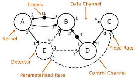
The behaviour of processes (kernels B, C and D) controlled by the same detector(s) (detector E) is correlated.
Behaviour
For explanatory purposes, it is convenient to introduce the term port, which refers to a point where some channel connects to a process. Control ports denote connections of control channels and the corresponding receiving process. On the other hand, input ports refer to ports from which processes receive tokens through data channels. Output ports are ports to (data or control) channels onto which a process produces tokens. SADF fixes the consumption rates corresponding to control ports to 1.
The behaviour of a kernel is merely determined by the scenario-valued tokens received via control ports. If a kernel has control ports, its firing starts with interpreting the first token on all its control ports after they have become available. The combination of their values determines the scenario in which the kernel will operate. In case no control channels are connected to a kernel, it behaves according to a default scenario. After establishing the scenario, which boils down to fixing the rates and execution time distribution, the kernel waits until sufficient tokens are available on its input ports conform the consumption rates. At the moment that sufficient tokens are available, the kernel performs its data processing behaviour by delaying for an amount of time that is gven by a sample drawn from the previously determined execution time distribution. Firing ends with removing the number of tokens from the (data and control) channels connected to it as specified by the consumption rates as well as producing the number of tokens to output ports conform the production rates. A kernel is said to be inactive in a scenario in case it does not consume and produce tokens from/to any input/output ports.
The firing of a detector also starts with determining the scenario. If a detector has control ports, the scenario is determined by interpreting the first token on all its control ports after they have become available (similar as for a kernel). An SADF graph including detectors with control ports is also said to incorporate hierarchical control. In case no control channels are connected to a detector, it behaves according to a default scenario. The effect of establishing the scenario for a detector differs however from determining the scenario in which a kernel will operate. A detector includes a (discrete-time) Markov chain (state machine where transitions are taken probabilistically) for each possible scenario in which it can operate. These Markov chains are used to determine the subscenario in which the detector will operate. The subscenario refers to certain consumption/production rates and an execution time distribution of the detector. Establishing the scenario for a detector merely fixes the Markov chain that will be used for determining the subscenario. Together with establishing the scenario, the subscenario is determined by the state of the involved Markov chain entered after making one transition. Together, scenario and subscenario fix the rates and execution time distribution. After establishing the scenario and subscenario, the detector waits until sufficient tokens are available on its input ports. At the moment that sufficient tokens are available, the detector performs its behaviour by delaying for an amount of time that is given by a sample drawn from the previously determined execution time distribution. Firing ends with removing the number of tokens from the (data and control) channels connected to it as specified by the consumtion rates and producing the number of tokens to output ports conform the production rates, where tokens produced onto control channels are valued.
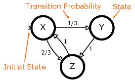
The behaviour of the involved detector and the processes it controls perfomed as a consequence of the first firing of the detector is determined by the subscenarios associated with states Y and Z.